
")
Acquiring torpedo firing data
Determining the parameters of the target’s course: the angle on the bow, speed, and possibly the distance, was a critical issue when launching torpedoes. Initially, the course was determined solely on the basis of visual observation. The main limitation of visual observation is the dependence on weather conditions and time of day/night. However, during the Second World War technical measures (radar and sonar) emerged, which allowed observation at night and in bad weather conditions.
There were three ways to determine the parameters on the basis of visual observation:
- estimating “by eye”
- by plotting
- acquisition of data from artillery control (larger vessels)
Target course parameters “by eye” estimation was the basic method, because it could be used in any situation and did not require any special equipment and was not time-consuming. The accuracy of the results depends on the experience of the person making the estimate.
The speed can be estimated on the basis of the size of the bow wave and wake. An additional clue – assuming correct target recognition – can be the range of speed that the target can cruise, read from the ships register. Another helpful piece of information for estimating speed, knowing the type of ship, could be the revolutions per minute (RPM) of the target ship’s propellers.
Angle on the bow – that is angle between target course and the line of target bearing – was estimated on the basis of an external view of the target – how much the sides of the superstructures were shortened, relative position of the deck equipment situated on both sides of the target vessel (cranes, heads of air intakes) and so on.
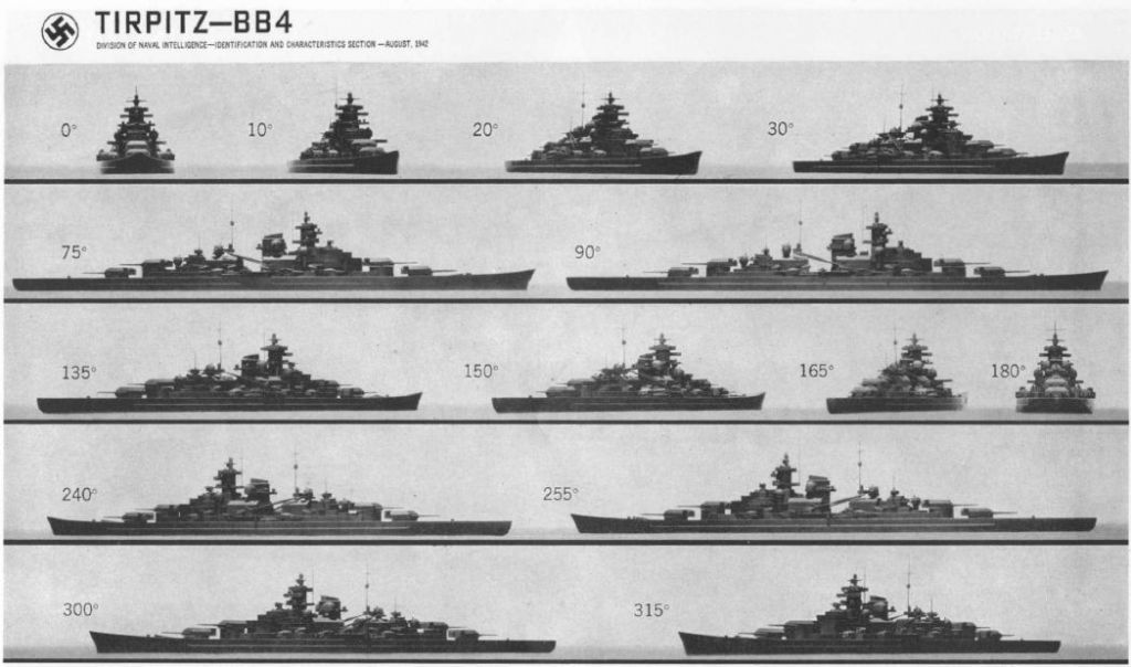
Information necessary for estimates was gathered from the annuals of warship and merchant vessel registers (i.e. Weyers Taschenbuch der Kriegsflotten, Die Handelsflotten der Welt, Handbuch der Schiffstypenkunde für die Kriegsmarine, Jane's Fighting Ships). Many of these books were published by various Naval Intelligence Offices. Sample pages prepared by the American Office Of Naval Intelligence which describe the German battleship Tirpitz contain (among other things) silhouettes of the warship as seen from different angles on the bow, dimensions of the hull (including height of the masts) and the relationship between propeller rotating speed (RPM) and knots per hour.


As mentioned earlier, this method was fast, but its accuracy depended on the experience of the person who evaluated the target course parameters. It was mainly used during an attack at close range, when the target's dynamic maneuvers prevented the use of more accurate but more time-consuming methods, and the short runtime of the torpedoes compensated for the errors in estimating the angle on bow and speed.
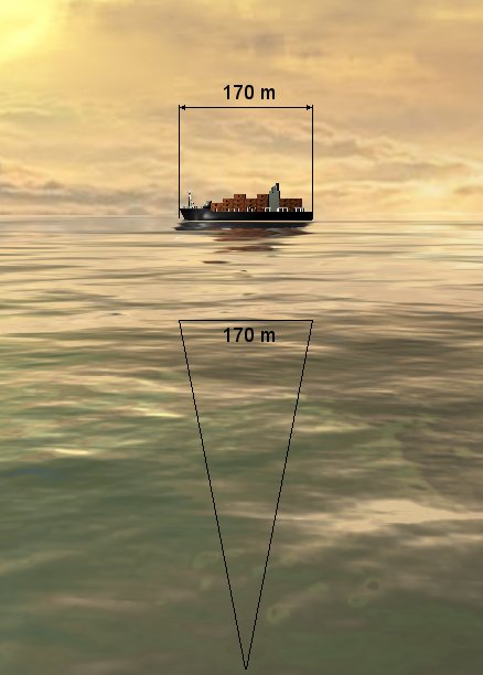
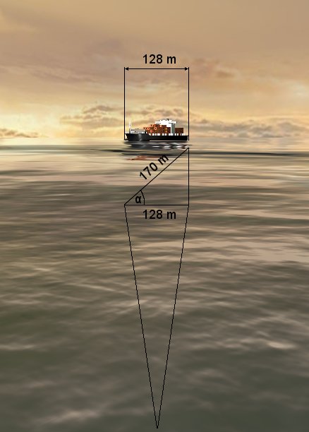
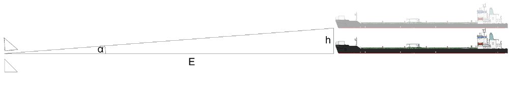
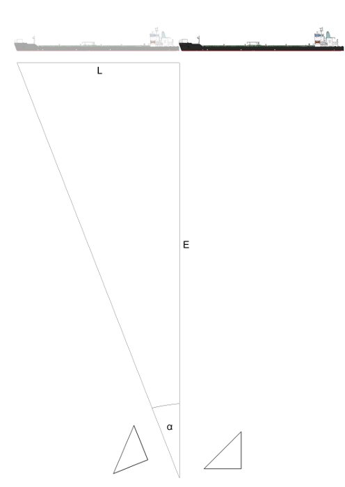
The angle on the bow can be quite accurately determined if you know the actual length of the target after measuring the visible target length (which can be smaller due to the position of the target with an angle on the bow different than 90°). However this method requires making some additional surveys. The idea is presented in the drawings below. The first drawing shows the target with the angle on the bow equal to 90° (port), and its visible length is (assume) Lz = 170 m – and is equal to its real length Lr. The second drawing presents the target with the angle on the bow equal to 49° (port) – its visible length is Lz = 128 m. Knowing the real length of the target (i.e. from merchant ships register), the angle on the bow can be calculated from the following formula:
\[\begin{aligned} γ = 90° - α = 90° - arc cos \frac{L_{z}}{L_{r}} = arc sin \frac{L_{z}}{L_{r}} \end{aligned} \]
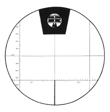
The simplest way to measure the length (and height) of the target was to use graticules that were embedded into periscopes and bridge night sights (Germ. UZO - U-Boot-Ziel-Optik, Eng. TBT - Target Bearing Transmitter). German periscopes constructed by the Zeiss company which were installed on the U-Boats during World War Two, were equipped with a graticule which had two scales: vertical - calibrated in angular mils, and horizontal – calibrated in degrees.
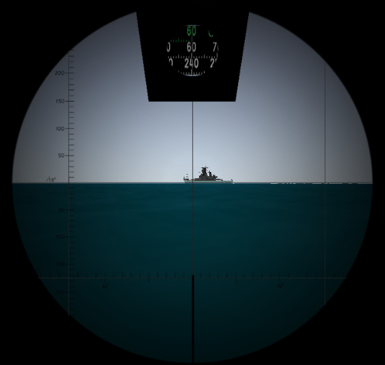
The distance to the target based on the target height was calculated as follows:
distance (kilometers) = target height (meters) / angular target height (angular mils)
For example, the distance to the sinking merchant ship visible in the photo is (assuming mast height equal to 20 meters):
20/120 = about 170 meters when periscope magnification is 1,5x and about 650 meters when magnification is 6x.
Knowing the distance to the target, the visible length of the target (which can be smaller than the real length due to the influence of the angle on the bow) can be calculated:
visible length of target (meters) = distance (meters) * tan (angular length of target in degrees)
Knowing the visible length of the target and its real length (from the merchant vessels register or annual of warships), the angle on the bow can be calculated using the formula given previously.
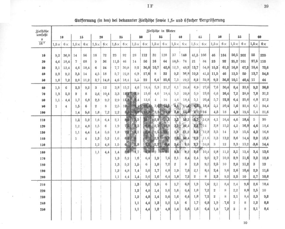
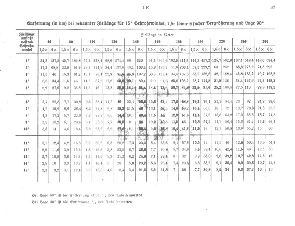
An addendum to the regulations M. Dv. 416 Torpedo-Schießvorschrift für U-Boote: the collection of tables M. Dv. 416 Tabellenheft zur Torpedo-Schießvorschrift für U-Boote contains two tables, which could be used for determining the distance. The first table contained the values of the distance to the target (in hm) depending on the measured height (in angular mils) and its assumed height in meters (for both magnifications: 1.5x and 6x). The second table contained the values of the distance to the target (in hm) depending on the measured length (in degrees) and its assumed length in meters (also for both magnifications: 1.5x and 6x). The table contains values for the angle on the bow 90°, but on the bottom of the page, there were notes, that for angle on the bow 50° and 30°, the distance was equal to ¾ and ½ of the value read from table.
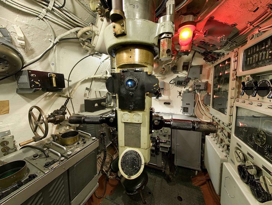
In the inter-war period, the companies manufacturing periscopes started to equip their scopes with rangefinders (Germ. Doppelbild-Entfernungsmesser, Eng. Stadimeter). Due to periscope construction (lack of the optical base), there cannot be coincidence or stereoscopic rangefinders. In fact, these were devices which facilitated the measurement of the angular height of the target. When the assumed target height was entered, the distance could be read from the appropriate dial. In the view field of a periscope equipped with such a rangefinder, two images of the target were visible – one above the other. Using a dedicated hand wheel, the upper image would be moved in such a way that the waterline of the upper image touched the top of the masts of the lower image. The upper image was moved by rotating an additional prism in the optical arrangement of the periscope. The amount of rotation of this prism relative to its initial position was equal to the angular height of the target and was shown on the rangefinder dial.

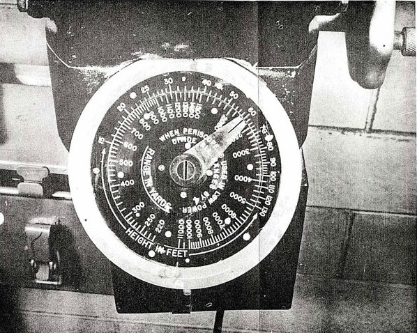
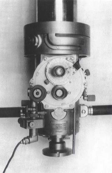
To avoid the necessity of making the calculation (dividing the height of the target by the tangent of the measured angle), the dial which showed the angle was built into the simple calculating instrument, similar to the circular slider. The photo below shows the dial of the American periscope type 92KA40T/1.99. The external dial is movable and is rotated along with the rotation of the prism (that is along the movement of the upper image). The internal dial is fixed. When both images are aligned properly, the distance to the target can be read against the correct target height from the internal dial.


Further modification of this rangefinder made possible measurement of the angle on the bow (Germ. Doppelbild-Entfernungs- und Zielkurswinkelschätzer, Eng. Range and course-angle finder). The trainable prism which created the second image can be rotated by 90°, so the movable image is at the same level as the primary image and can be moved horizontally. That enables measurement of the angular length of target.
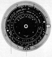
The rangefinder of the American type 91KA40T/1.414HA (Type II) attack periscope consisted of three concentric dials. The trainable, external dial had two scales: one on its outer edge, in feet, indicating the length of the target and second – on its inner edge, in degrees, indicating the target angle on the bow. The middle dial's scale was in yards and indicated the range to the target. The middle dial rotated along with the rotation of the prism which created the second image. The internal dial’s was in feet and indicated the target height.
The distance to the target and target's angle on the bow was measured as follows: the length of the target read from the merchant ship or warship register was entered by rotating the external dial such that the proper target length was indicated by a stationary mark on the bottom of the dial. Initially, both images, stationary and movable, created by the trainable prism overlapped. Then, using the regulating knob coupled with the trainable prism, the images were split. The operator adjusted the images such that the water line of the upper image touched the top of the masts of the lower image. The image was moved because when the prism was rotated the middle dial was rotated too. When both images were adjusted properly, the distance to the target was read from the middle dial against the known target height on the internal dial.
Next, to measure the angle on the bow, the image splitting was continued till the moment when the movable image disappeared out of the upper edge of the view field and the regulating knob reached its limit position. At that time, the gear rotated the prism to the position where the image could be moved horizontally. Using the regulating knob, training in the opposite direction, the image entered the view field from the left side (on the same level as the still image) and moved towards the still image. When the stern of the movable image touched the bow of the still image, the angle on the bow could be read from the external dial against the distance measured in the previous step.
With continued training of the regulating knob, both images overlapped again. When the regulating knob reached its limit position the gear rotated the prism to its initial position (that is to the position, where the image could be moved horizontally again) and the distance and angle on the bow measurement could be performed again.
on American submarines of the Gato and Balao classes [7]
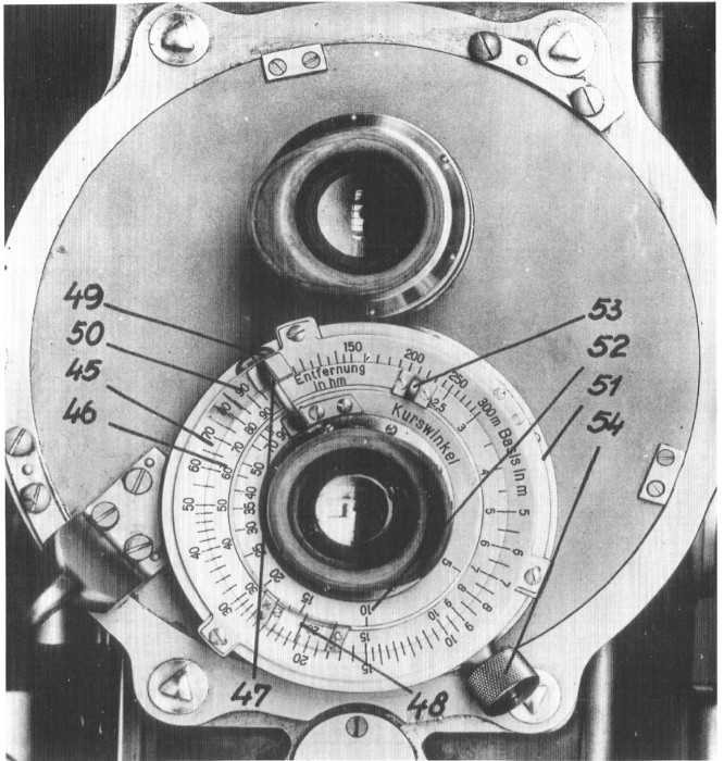
The rangefinder of the German type ASR C/6 attack periscope consisted of an external, non-movable dial (45) (Basis), with its scale in meters, a trainable middle dial (46) (Entfernung) whose scale was in hectometers and a trainable internal dial (52) (Kurswinkel) with its scale in degrees. The middle dial rotated along with the rotation of the prism, which created a second image. The inner dial was rotated by means of the handle (47). The indicator (50) was attached to the handle (47) which allowed for reading the values from the external dial corresponding to the angle 90° on the internal dial. An additional indicator (48) facilitated reading the values from the middle and external dials. It was rotated by means of the handle (53).
The distance to the target and the target's angle on the bow was measured as follows: the height of the target read from the merchant ship or warship register was set on the external dial by means of the indicator (48), and the length of the target – by means of the indicator (50). Initially, both images, stationary and movable, created by the trainable prism overlapped. Then, using the regulating knob coupled with the trainable prism, the images were split. The operator adjusted the images such that the water line of the upper image touched the top of the masts of the lower image. The image was moved because when the prism was rotated the middle dial was rotated too. When both images were adjusted properly, the distance to the target was shown by indicator (48) on the middle dial (46). It should be noted, that indicator (48) has not changed since its initial setup – the middle dial was trained under the indicator.
Next, to measure the angle on the bow, the image splitting was continued till the moment when the movable image disappeared out of the upper edge of the view field and the regulating knob reached its limit position. At that time, the gear rotated the prism to the position where the image could be moved horizontally. Using the regulating knob, training in the opposite direction, the image entered the view field from the left side (on the same level as the still image) and moved towards the still image. When the stern of the movable image touched the bow of the still image, the angle on the bow could be read from the internal dial against the distance measured in the previous step.
With continued training of the regulating knob, both images overlapped again. When the regulating knob reached its limit position the gear rotated the prism to its initial position (that is to the position, where the image could be moved horizontally again) and the distance and angle on the bow measurement could be performed again.
A demonstration showing the operation of this rangefinder is available here.
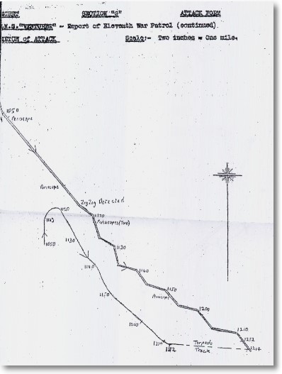
The plot (Germ. Koppelverfahren) was another method to determine the parameters of the target's course. It consists of making a few distance measurements together with bearings and drawing it on a chart (together with the position of own ship). A sample plot is presented in the drawing below.
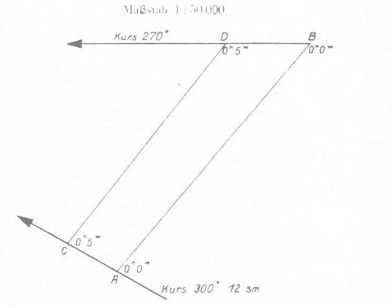
At 0h0m own ship is at the point A, its speed is 12 knots, its course is 300°, target bearing is 40° and distance to the target is 10400 m.
At 0h5m the target bearing is 38° and distance to the target is 8900 m.
These positions were drawn on the plot in the scale of 1:50000. First, the position of own ship was drawn at point A. Then, from this point, the target bearing line was drawn at an angle of 40°, and at a distance of 20,8 cm the position of the target was drawn (at point B).
Next, from point A, the own ship course line was drawn at an angle of 300° and its position marked (point C) on the plot at 0h5m at a distance of 3,7 cm (distance covered in 5 minutes at the speed of 12 knots, scaled down to 1:50000). From point C, the target bearing line was drawn at an angle of 38° and at a distance of 17,8 cm its position is marked on the plot (point D).
Connecting points B and D, the target course line is determined, and can be measured – it is equal to 270°. The distance between these points was covered by the target in 5 minutes. This distance is equal to 5,6 cm and that works out to be 2800 meters. That means, that the target is moving at a speed of 18 knots. Knowing target course, target bearing and own course, the angle on the bow can be easily determined by measuring its value on the plot (by means of protractor), or using the formula (angle on the bow = target course ± target true bearing) or using calculating discs called Is-Was (Germ. Lagenwinkelscheibe).
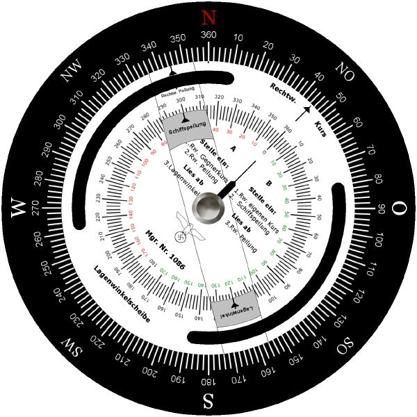
German Lagenwinkelscheibe consisted of three coaxial dials: external compass dial (1), internal dial (2) and transparent dial with reading line (3). The compass dial is graduated from 0 to 360°. The internal dial is graduated from 0 up to 180° and then down to 0. Arrow (4) on the 0 mark is pointed outside. The reading line (3) has three marks which allows setting or reading the target's true bearing (5), target relative bearing (6) and angle on the bow (7).
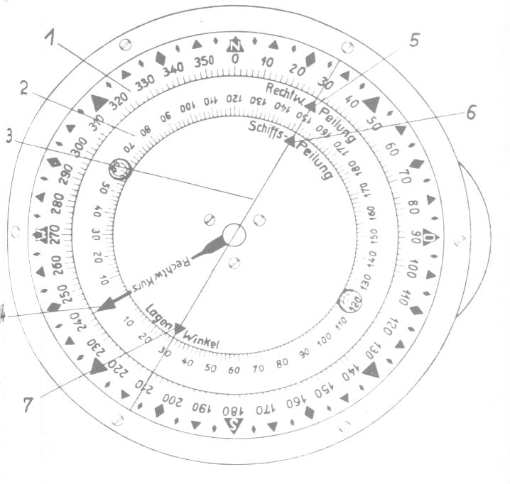
To determine angle on the bow, the following steps should be performed:
1. Setting target true bearing – by rotating the transparent dial, the mark (5) should point to the proper value on the compass dial (1)
2. Setting target course – by rotating internal dial (2) the arrow (4) should point to the proper value on the compass dial (1)
3. The angle on the bow is pointed to by mark (7) on the internal dial (2).
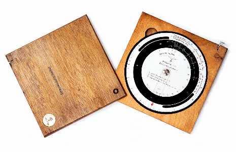
Demonstration showing the operation of such calculating disc is available here.
In fact, further measurements needed for plot were taken more frequently (about every 30 seconds). The more measurements that were made, the more accurate the results achieved. The method was time-consuming, (minimum time of plotting that allowed for determining target course parameters was about 5 minutes), but its accuracy allowed for instance for detecting the zigzag pattern of the target.
To determine target bearing, various optical bearing finders (i.e. TUZA - Torpedo-U-Boot-Zielapparat, UZO – U-Boot-Ziel-Optik) or periscopes were used. The distances were measured by determining angles (i.e. angle height) - by means of graticules or prism rangefinders.
The plot was used not only for determining the course of single targets, but also groups of warships or convoys. A torpedo attack launched on the basis of a plot was recommended in good visibility conditions; that is mainly in daylight.
In the case of larger warships it was possible to acquire target course parameters from the artillery fire control room, where these were calculated by means of artillery fire control computers, which in turn were fed by data gathered by artillery rangefinders and directors.
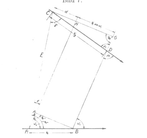
In the mid-war period Germans developed a torpedo firing method called Ausdampfverfahren. It was based on adjusting own ship course and speed such that the target bearing remains constant (its changes were suppressed, Germ. Ausgedampft). The concept is presented on the drawing below.
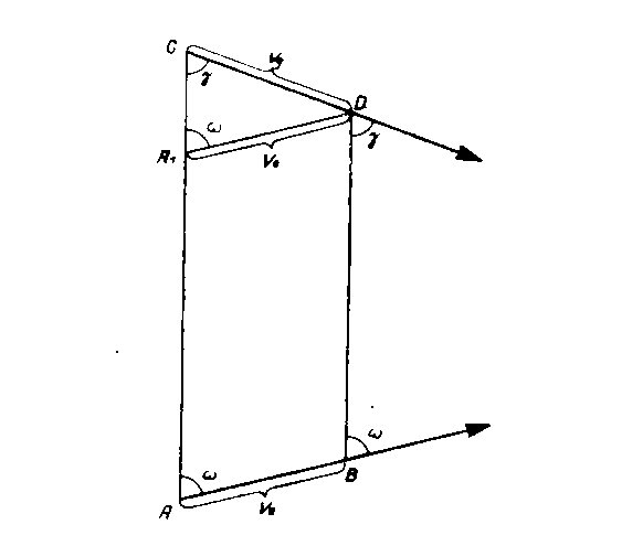
Vector AB shows own ship course. Its speed is equal to ve. The target course is represented by vector CD, and target speed is vg. The own ship speed is so adjusted that target bearing ω (at the points A and B) is constant. The angle on the bow γ at the points C and D is equal.
The torpedo director determines deflection angle β using the law of sines:
where vg and γ are unknown.
On the drawing, the segment A1D is parallel to segment AB and its length is equal to the length of segment AB that is equal to the speed of own ship ve. The angle near the vertex A1 is equal to ω.
The law of sines applied to the triangle A1CD:
The right side of this equation (own speed and target bearing) are known, so they can be inserted directly in the numerator of the previous formula, which gives:
In practice, attacks developed using this method required setting course and speed of own ship in such a way that the target bearing would remain the same. On the torpedo director, the target speed was set to own ship speed, and the angle on the bow was set to the target bearing. Then the ship started a turn (in case of fixed torpedo tubes) and torpedoes were launched when the target crossed the aiming line. In the case of trainable torpedo tubes, the aiming was done by training the tubes.
This method was recommended at dusk and at night. It did not require the measurement of distance, but only adjusting own speed and course, which usually took up to 10 minutes.
The main disadvantage of the Ausdampfverfahren method was the relatively long time needed for suppressing changes of target bearing. That's why, on the basis of this method, another procedure was developed, the so called Auswanderungsverfahren method. This procedure was less accurate than Ausdampfverfahren, but required taking only two target bearings 1 minute apart and measuring (or estimating) the distance to the target during the taking of the first bearing.
There were two versions of this method: Auswanderungsverfahren “A” and Auswanderungsverfahren “B”.
The concept of the “A” version is shown in the drawing below:
Own ship course is presented as line AB, own ship speed is ve. The target course is shown by line CD, and its speed is vg. In 1 minute own ship moves from point A to point B, and the target moves from point C to point D. The target bearing at point A is ω, and at point B is ω1, that means that it is altered by value ε. In other words, in 1 minute the target bearing was altered by angle ε.
The torpedo director determined deflection angle β using the law of sines:
where vg and γ1 are unknown.
From the drawing one can see, that segment CD1 is parallel to segment AB, and segment BB1 is parallel to segment AC, so length of segment CB1 = AB = ve, and B1D1 is equal to the linear change of target d. Length of segment is CD1 = ve + d, the angle at the vertex D1 is equal to ω1.
The angle ω1, own ship speed ve and linear change d is known, so the law of sines can be applied to the triangle CDD1:
After inserting the right side of the above equation directly in the numerator of the previous equation, the result is:
On the torpedo director the target speed was set to own ship speed (with the correction for linear change d) and the angle on the bow was set to the target bearing ω1. The decision as to whether the linear change d had to be added to or subtracted from the own speed ve depended on whether the target bearing increased or decreased after 1 minute.
Then the ship started its turn (in the case of fixed torpedo tubes) and torpedoes were launched when the target crossed the aiming line. In the case of trainable torpedo tubes, the aiming was done by training the tubes.
During the taking of the first target bearing, the distance to target E was also measured (or estimated). After 1 minute, another target bearing was taken and the difference was calculated: ε = ω – ω1. The linear change d was calculated using the law of sines applied to triangle BB1D1:
Because the value d is in knots, and the distance E is measured in hectometres, the distance E should be multiplied by the factor 100*60/1820.
In practice calculating the linear change d was done by means of a calculating disc known as Rundschieber für Auswanderungsverfahren “A”. It was kind of a circular sliding rule which consisted of three dials and four scales. External and internal dials were fixed, the middle dial was trainable.
To calculate the result, the external and middle dials should be set in such a way, that angle ω1 on the middle dial was against the angle ε on the external dial. The linear change d was read from the internal dial, against the respective distance E on the middle dial.
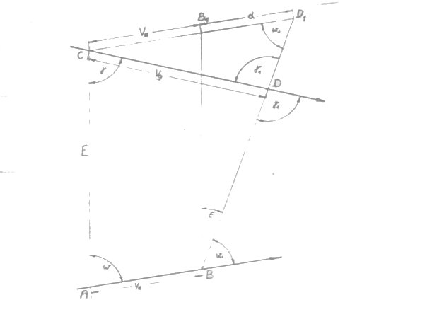
The concept of the “B” version is shown in the drawing below:
While in version “A” the linear change was projected on the line which was parallel to the course of own ship. In version “B” this linear change was projected on the line which was perpendicular to the line of the second target bearing.
Own course is shown by line AB, own speed is equal to ve, the target course is shown by line CD, and its speed is equal to vg. During 1 minute, own ship moves from point A to point B and the target ship from point C to point D. The target bearing at point A is equal to ω, while at point B is equal to ω1 that means it is altered by value ε.
The torpedo director determined deflection angle β using the law of sines:
where vg and γ1 are unknown.
Because triangle CGD is the right triangle, there is the relationship:
The segment CG is target speed projected on the line perpendicular to the line of the target bearing.
The length of segment CG is equal to GH + HC = GH + d. Both values GH and d have to be calculated.
In the right triangle BA1A there is following relationship:
So
The segment GH is own speed projected on the line perpendicular to the target bearing.
The length of segment d can be calculated from the formula:
So the law of sines applied to the torpedo triangle appears as:
It is equal to:
On the torpedo director the target speed was set to the component of own speed (with the correction for the linear change d) and the angle on the bow was set to 90°. The decision as to whether linear change d has to be added to or subtracted from the component of own speed vk depends on whether the target bearing increased or decreased after 1 minute.
Then the ship started a turn (in the case of fixed torpedo tubes) and torpedoes were launched when the target crossed the aiming line. In the case of trainable torpedo tubes, the aiming was done by training the tubes.
As with version “A”, during the taking of the first target bearing, the distance to target E was measured (or estimated). After 1 minute, another target bearing was taken and the difference was calculated: ε = ω – ω1.
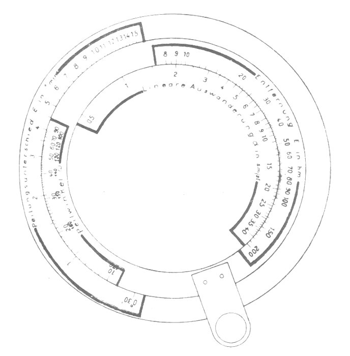
The component of own speed vk and linear change d was calculated by means of a calculating disc, the so called Rundschieber für Auswanderungsverfahren “B”. On both sides of the disc were scales for determining the speed component and linear change.
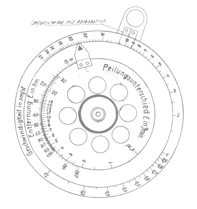

A scale for setting own ship speed ve and a trainable internal dial with the scale for setting target bearing ω1 are located on the front side of the disc, on its external edge. A handle is attached to the trainable internal dial that has a pointer on its rear side for reading the speed component vk.
On the rear side of the disc, on the fixed external edge are two scales – one for reading the component of own speed vk , and the other for reading the linear change d. On the fixed part of the disc – but close to the center – is the scale for setting the distance to target E. The scale for setting angle ε is located on the internal, trainable dial. The pointer for reading the linear change d on the external dial is attached to this dial.
Version “B” of the Auswanderungsverfahren method (in short Aw-Verfahren B) was the recommended version to use. Version “B” appears to be more complicated than Version “A” as it required performing two calculations, but it appears it was less prone to errors - the angle on the bow on the torpedo director was always fixed and equal to 90°.
Comparison of different methods of determining target course data
| Method | Measured values | Time-consumption | Accuracy | Required additional equipment | Notes |
| Estimation | N/A | N/A | low | N/A | Backup method |
| Plot | distance, bearing | min 10 minutes | high | N/A | N/A |
| Ausdampfverfahren | bearing, own speed | ~ 10-15 minutes | high | N/A | N/A |
| Auswanderungsverfahren | bearing, own speed, distance | ~ 1 minutes | medium | calculating discs | N/A |
It should be noted that despite these methods having been developed during a time when torpedo fire was controlled by simple torpedo directors, they were so universal that they were also used later during World War II when sophisticated torpedo computers like the Siemens TVRe S2 were in service.
Summary of torpedo attacks and methods of determining
target course data during World War II [16]
| U-Boat | Date | Method | Target |
Torpedoes fired/hit |
| U 47 | 11.12.1939 | Ausdampfverfahren | no data | 2/0 |
| U 47 | 12.12.1939 | Ausdampfverfahren | no data | 2/0 |
| U 48 | 11.10.1940 | Estimation | Brandanger | 1/1 |
| U 48 | 11.10.1940 | Estimation | Port Gisborne | 1/1 |
| U 48 | 11.10.1940 | Estimation | no data | 1/0 |
| U 48 | 11.10.1940 | Estimation | no data | 1/0 |
| U 48 | 12.10.1940 | Estimation | Davanger | 1/1 |
| U 48 | 17.10.1940 | Estimation | Scoresby | 1/1 |
| U 48 | 17.10.1940 | Estimation | Languedoc | 1/1 |
| U 48 | 17.10.1940 | Estimation | no data | 1/0 |
| U 48 | 18.10.1940 | Estimation | Sandsend | 1/1 |
| U 48 | 18.10.1940 | Estimation | no data | 1/0 |
| U 48 | 20.10.1940 | Estimation | Shirak | 1/1 |
| U 100 | 8.12.1940 | Estimation | no data | 1/0 |
| U 100 | 8.12.1940 | Estimation | no data | 1/0 |
| U 100 | 14.12.1940 | Estimation | Kyleglen | 1/1 |
| U 100 | 14.12.1940 | Estimation | Euphorbia | 1/1 |
| U 100 | 14.12.1940 | Estimation | no data | 1/0 |
| U 100 | 14.12.1940 | Estimation | no data | 1/0 |
| U 100 | 14.12.1940 | Estimation | no data | 1/0 |
| U 100 | 18.12.1940 | Estimation | Napier Star | 2/1 |
| U 100 | 18.12.1940 | Estimation | no data | 1/0 |
| U 100 | 22.12.1940 | Estimation | no data | 2/0 |
| U 138 | 16.09.1940 | Ausdampfverfahren | no data | 1/0 |
| U 138 | 20.09.1940 | Szacowanie | New Sevilla | 1/1 |
| U 138 | 20.09.1940 | Szacowanie | Boka | 1/1 |
| U 138 | 20.09.1940 | Szacowanie | City of Simla | 1/1 |
| U 138 | 21.09.1940 | Ausdampfverfahren | Empire Adventure | 1/1 |
| U 435 | 17.03.1943 | Estimation | William Eustis | 2/1 |
| U 435 | 17.03.1943 | Estimation | no data | 2/0 |
| U 435 | 17.03.1943 | Estimation | no data | 2/0 |
| U 435 | 17.03.1943 | Estimation | no data | 1/0 |
| U 552 | 1.11.1941 | Ausdampfverfahren | no data | 4/0 |
| U 552 | 1.11.1941 | Estimation, speed on basis propellers RPM |
no data | 2/0 |
| U 557 | 29.05.1941 | Ausdampfverfahren | Empire Storm | 1/1 |
| U 557 | 29.05.1941 | Ausdampfverfahren | no data | 1/0 |
| U 557 | 27.08.1941 | Ausdampfverfahren | Segundo | 1/1 |
| U 557 | 27.08.1941 | Ausdampfverfahren | Saugor | 1/1 |
| U 557 | 27.08.1941 | Estimation | no data | 1/0 |
| U 557 | 27.08.1941 | Estimation | no data | 1/0 |
| U 557 | 27.08.1941 | Estimation | no data | 1/0 |
| U 557 | 27.08.1941 | Estimation | Tremoda | 1/1 |
| U 557 | 27.08.1941 | Estimation | no data | 1/0 |
| U 557 | 27.08.1941 | Estimation | Embassage | 1/1 |
| U 628 | 17.04.1943 | Estimation | Fort Rampart | 3/2 |
| U 628 | 5.05.1943 | Plot | Harbury | 5/1 |
| U 628 | 5.05.1943 | Estimation | no data | 1/0 |
| U 952 | 26.02.1944 | Estimation, speed on basis propellers RPM |
no data | 1/0 |
| U 952 | 26.02.1944 | Estimation | no data | 1/0 |
| U 952 | 28.02.1944 | Estimation | no data | 2/0 |
| U 952 | 4.03.1944 | Estimation | no data | 1/0 |
| U 952 | 10.03.1944 | Estimation | no data | 3/0 |
| U 952 | 10.03.1944 | Estimation, speed on basis propellers RPM |
Wiliam B. Woods | 1/1 |
| U 967 | 26.04.1944 | Estimation, speed on basis propellers RPM |
no data | 1/0 |
| U 967 | 5.05.1944 | Estimation, speed on basis propellers RPM |
USS Fechteler | 1/1 |
| U 967 | 5.05.1944 | Estimation | no data | 1/0 |
| U 967 | 8.05.1944 | Estimation, speed on basis propellers RPM |
no data | 1/0 |
References:
[1] ONI-204 GERMAN NAVAL VESSELS
[2] Die Deutsche Wochenschau No 596, 1942
[3] Die Deutsche Wochenschau
[4] Harry Schlemmer, Vom Turmsehrohr zum Optronikmast. Geschichte der Zeiss U-Boot-Sehrohre
[5] Tabellenheft zur Torpedo-Schießvorschrift für U-Boote, 1940
[6] Submarine torpedo fire conrol manual - Duties of the Fire Control Party
[7] Submarine Periscope Manual, Range and Course-Angle Finder
[8] Hans Techel, Der Bau von Unterseebooten
[9] USS Pampanito virtual tour - conning tower
[10] Richard Lakowski, Deutsche U-Boote GEHEIM 1935-1945
[11] Vesikko - Periscope
[12] Torpedoschießvorschrift, Heft 2, Ermittlung der Schußwerte, 1930
[13] Museum of World War II - German Military Collection
[14] Subsim - Kriegsmarine Wiz-Wheel templates released!
[15] HMS Venturer, Report of Eleventh War Patrol, 1944
[16] Torpedo Schußmeldungen